


EUR
en
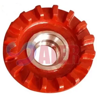
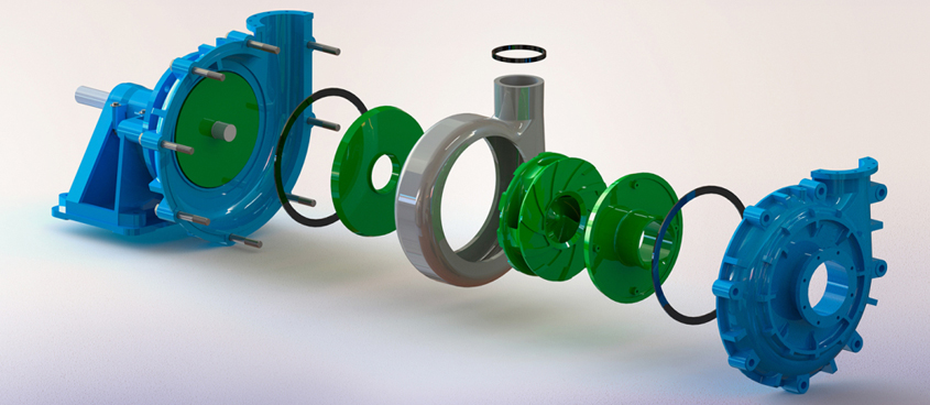
The flexible vane (impeller) pump has a cam shape between the suction and discharge ports on the inside diameter of its housing. An impeller with flexible blades rotates in this housing. When each blade passes the discharge port, it is depressed radially inward, which forces fluid to discharge. When it passes the cam and the vane straightens out radially again a slight vacuum is created which induces the fluid from the inlet into the displacement volume between it and the following blade. These pumps have a gentle action and are used extensively in the food industry. They are self-priming and are used on large capacity applications. The maximum pressure capability of the pump is in the order of 10 kp a(70 psi) because of the non-rigid displacement volumes. This same property also eliminates the need for a relief device. Dry running for short periods (a minute or less) can be accommodated. Maximum operating temperatures are a function of the liner material, and generally in the range of 80–100°C. Like lip seals the blade tips should be prelubricated before initial use. Some applications are food, beverage, milk and dairy products, pharmaceutical, chemical marine engine cooling, entrained air containing products etc.
Generally, groundwater is sampled from filters in groundwater wells, where it is usually pumped up with an impeller pump. Before sampling, the filters are cleaned with the groundwater to be sampled. The volume of water used for cleaning is about three times the void volume of the filter and connection tube. Applying an under pressure to the well collects samples using this procedure. Often, solute gases like carbon dioxide are expelled, causing the pH of the sample to rise. Next, the sample is filtrated; for example, through a 0.45 μm pore size cellulose nitrate membrane filter. Although it is internationally accepted that a pore size of 0.45 μm can distinguish between suspended and solute substances, colloidal particles have been shown to cause problems here. These particles are solid and can easily slip through the 0.45 μm membrane filters. The sorption of substances is also unpredictable when using filters. Furthermore, the transport of samples to the laboratory takes place under unconditioned circumstances and transport times are often long and variable. The pH shift, filtration, and variable transport times cause drastic changes in the chemical composition of the sample. The changes restrict the representativeness of the sample of groundwater originally present in the well.
Although the representativeness of the original groundwater may be poor, samples are still analyzed to obtain an impression of the condition of the groundwater. Since the chemical composition of groundwater highly resembles the composition of drinking water, groundwater is analyzed in almost the same way as drinking water. However, tritium is usually not measured when drinking water is analyzed. Tritium in groundwater can be used to assess the time groundwater needs to infiltrate the soil from surface level to the filter of a well. Tritium found in groundwater originates from nuclear tests carried out from 1962 to 1965 (highest in 1963). Having been washed from the atmosphere through precipitation, the tritium ended up in groundwater. As the decay time of tritium is 12.43 years, its activity can be measured over a long time period. Transport times can be calculated from the time series for tritium monitored in a well filter. Although these transport times can be assessed from individual measurements, the accuracy is then much less. Tritium is measured through the decay products, electrons, and helium. Normally, beta radiation is measured to establish the concentration of tritium. Water containing tritium is concentrated to improve the accuracy of the measurements in groundwater. First, a portion of the sample is distilled to remove contaminants. This is followed by enrichment during a 5-day electrolysis of the sample. Sodium hydroxide is added to 150 ml of the sample to increase the conductivity. The sample is then placed in an electrolysis cell, and cooled in a freezer. To prevent absorption of water from the ambient air, the electrolysis cell is trapped on a zeolite absorption column. After electrolysis, 15 ml of the sample remains. This is converted to hydrogen through the reaction with elemental magnesium. The resulting tritium-containing hydrogen gas is catalytically converted with ethene to ethane, using platinum as catalyst. The gas is then brought into a proportional counter and activity counted. On each run, both a background sample and a sample with known activity are analyzed. An alternative way is to add the sample to a portion of degassed water and leave the sample aside for about half a year. Helium is formed and can be measured by mass spectrometry. From the result the amount of tritium original present the tritium concentration is derived.
The loaded-carbon grade and the precious-metal extraction efficiencies dictate the rate of carbon movement required. Carbon is generally advanced by either airlift (for smaller plants) or by recessed impeller pumps. The plant design must take into consideration the impact of the return slurry flow from carbon advance on the intertank screen capacity. For average-grade gold plants this is not an issue. However, for ore with a high silver grade, the carbon movement may be significant. This can lead to large slurry flows coming from carbon movement. In this situation, separate carbon-transfer screens may be included to allow the slurry to return to the tank from where it came while still allowing the carbon to advance.
General troubleshooting guidelines are provided for process water storage tanks. Such tanks act as equilibrium tanks for receiving water from upstream equipment and supplying water to downstream equipment or other equipment in the plant. The tanks are always supplied with level switches and or level transmitters to start or shut-off upstream/downstream equipment, e.g. shutdown the process transfer pumps to protect the pumps from running dry and getting damaged or preventing tank overflow.
The retention of the particles can take place on the external layer of the granular medium (sand, anthracite, etc.), on which the water falls or is deep within the porous mass. The mechanisms of action are diverse. In depth, various types of forces work which cause the retention of the particles. In addition to the simple relationship, molecular, chemical, and surface forces work. Since the liquid conductor through the filter medium could be gravity or an impeller pump and, depending on one or the other, we speak of gravity filters, generally open, and pressure filters, continuously closed. The speed of passage of the water is directly proportional to the driving force or inversely proportional to the joint resistance of the filter medium and the retained surfaces. As the retained pavements accumulate, the pressure drop through the filter increases. If the available load is constant, the filtration speed decreases. If there is a device to vary the available load, a constant filtration speed can be maintained. The two ways of working have their concrete advantages. The optimal design of a filter should consider the following:•the size of the medium and the height of the width•filtration speed•available pressure•the way of filtering.
In filters with a granular medium, the way the pressure drop changes all the time is characteristic of the way the filter operates. An almost linear alteration of the discharge loss versus time or the total volume of the filtered water suggests a depth filtration. The waters that show a superficial filtration give a curve that corresponds to the exponential type in the stability between a few cycles of the longest viable duration and a good quality of the water; a size of the filter medium that is close to the optimal conditions is sought. There are filters designed with cycles between less than 10 and well over 24 h. The duration of the filtration cycles can be optimized in terms of the functionality of the number of filters in parallel and in conjunction with the dimensioning of the washing water storage tank. To wash the filters, once the pressure drop is excessive, or the quality deteriorates, it is done by means of a counter current. The retained pavements are displaced and dragged out of the filter with the water and are able to start the period again.
During the mid-1990s, DOE began the Advanced Hydropower Turbine System (AHTS) program as part of the Hydropower Program. The goal of the AHTS program is to develop environmentally friendly turbines. DOE funded the conceptual designs of four turbine types: three by Voith–Siemens and one by the team of Alden Research Laboratory (ARL) and Northern Research and Engineering Corporation (NREC). Voith–Siemens looked at redesigning a Kaplan and Francis turbine and developing a dissolved oxygen-enhancing turbine. ARL redesigned a pump impeller, used in the food processing industry to pump tomatoes and fish, to be used as a turbine.
The ARL–NREC design proceeded into the proof-of-concept stage, where the biological and engineering tests were finalized. Part of the proof of concept was to verify the biological design assumptions and the issue of whether the results of biological testing of a smaller model can be scaled upward to a full-sized turbine.
Many turbine manufacturers have begun designing environmentally friendly turbines, based on a potential market not only in the United States but also worldwide. In 2002, DOE selected three projects where environmentally friendly turbines will be installed and tested. Two projects involve improving downstream fish passage, and one involves increasing dissolved oxygen in discharged water.
The turbochargers were first used in the late 1980s and more widely adopted in the 1990s. The turbocharger device recovers hydraulic energy from the high-pressure brine (concentrate) stream in the reverse osmosis (RO) process and transfers that energy to a feed stream. The feed stream may be seawater going into a single-stage RO membrane block, or it may be first-stage brine stream being boosted in pressure for a second-stage membrane block for further recovery of permeate or flux balancing.
The turbocharger device consists of a pump section and a turbine section. Both pump and turbine sections each contain a single-stage impeller. The turbocharger incorporates a number of features designed to ensure simple operation, long operating life, reliable performance, and high availability. A nozzle directs the flow of water into the turbine side which then energizes the turbine impeller. The turbine impeller extracts hydraulic energy from the brine stream and converts it into mechanical energy. The pump impeller converts the mechanical energy produced by the turbine impeller back to pressure energy in the feed stream.
The process fluid provides all required bearing lubrication eliminating any external oil or grease requirements.
The turbocharger provides partial boost of the full feed flow to the membrane system. It can be thought of as a second pump in parallel with the HPP driven by a turbine instead of an electric motor.
_Brine pressure control_: The turbocharger can discharge brine against a back pressure. The unit does not require a brine disposal pump as is required by the Pelton wheel.
As is typical for all centrifugal devices, the turbocharger efficiency increases as flow capacity increases. The relative efficiencies between the turbocharger and the Pelton wheel can be seen in Fig. 11.5 B. It is important to keep in mind that the gap can be even larger since turbochargers are customer machines to optimize efficiencies while Pelton wheel use standard hydraulic designs.
The turbocharger device is equipped with a primary nozzle, a secondary auxiliary nozzle (AN), and an auxiliary nozzle control valve (ANCV) as shown in Fig. 11.6. The primary nozzle is sized to provide a concentrate system resistance (concentrate pressure) equal to the maximum design pressure at the design concentrate brine flow rate. The ANCV controls flow to AN in the turbine casing. The ANCV can accommodate a 5%–15% brine pressure variation at a constant brine flow, should the system conditions require it.
The ANCV does not bypass flow around the turbocharger. It is a unique way to achieve variable area nozzle flow without the energy wasting throttling and bypassing valve arrangements needed by Francis turbines/reverse running pumps.
According to previous year's research and comparison of current technology, the ozone sterilizer used in the drinking water treatment system is just like the one that is used in the water treatment plant but at a smaller scale. There are three main components: ozone generation, contact (state between generator and water storage), and storage. At the ozone generation part, the company either use traditional dielectric barrier discharge generator or upgrade to microplasma-based ozone generator, which has a higher cost but higher efficiency. The generator is connected to an air pump with an air drier, an upgrade at this part is it can use a pure compressed oxygen tank rather than using direct air. It can dramatically increase the production rate of ozone and avoid other potential oxidation compounds. However, it may take more space, frequent replacement of its parts and maintenance.
The second part is the contacting part, the main challenge for this part is to disperse the ozone gas into the smaller bubble to increase the contacting time and surface area. There are mainly two methods that can be used. One is using a nano air stone, placing it at the bottom of the reaction tank and allow the bubble to float from the bottom up to the top of the tank and assists in dissolving ozone in the water during this stage. Another method is using a pump that contains a needle wheel impeller, just like a protein skimmer or CO 2 disperser; it pumps air and ozone gas together through a needle wheel impeller pump, which disperses the gas into the fine bubble and mixes with water thoroughly. The reaction chamber can either be a tank or a tube depending on the space limitation and mixing efficiency. For example, in the normal water treatment plant, when there is enough space, they can build a big reaction chamber, which increase the contacting time of ozone and maximize the sterilization efficiency. But due to limitation of space in a modular water treatment system, it can be inconvenient to build a large reaction chamber in a moveable container. Hence, for this situation, a reaction tube can be applied, which can do the same job and would save more space too. However, due to a variety of water flow rate and limitation of contacting time, the ozone dosage can also be varied to maintain a constant degree of sterilization. But since the ozone residual will cause respiratory symptoms and mucous membrane irritation in a pool ventilated environment, it is necessary to discharge or recycle the undissolved ozone. To maximize the efficiency in using resources, it is a good idea to pump these ozone residuals back into the reactor or generator to use it again, especially in the modular water treatment system when space and resources are limited.
The final stage is the storing stage. The posttreated drinking water is collected here. Unlike chlorination, ozonation does not produce a residual that persists during water storage. It will make water susceptible to recontamination, so the container should have high sealing performance. Another optional upgrade is applying an active carbon filtration mechanism before the water feed into the container. Since the ozonation of metal or organic compound will potentially form precipitate or colloidal flocs, which eventually need to be removed before drinking. The frequency of replacing the filter media can be related to the pretreatment of the water. If the pretreated water has high hardness, it can form a high amount of precipitation during the ozonation, which will cause a frequent replacement of the filter media. For example, if applying a modular treatment system in the southern part of China, where most of the water sources are lower in hardness (ground surface water), it may not need extra pre-treatment methods to soft the water. This way, not only more space could be saved in the container but also can cut the budget of the capital cost of the installation. In those, low hardness water areas only replace the poststerilized filter media periodically may be enough for daily maintenance. However, if the modular treatment system has been applied someplace like Guelph or Beijing where most of the water sources are underground water with high hardness, then a pretreatment method is necessary to maintain the proper function of the system and prevent fast blockage of filter media.
It is important to recognize that a centrifugal _pump will operate only along its performance curve_. External conditions will adjust themselves, or must be adjusted in order to obtain stable operation. Each pump operates within a system, and the conditions can be anticipated if each component part is properly examined. The system consists of the friction losses of the suction and the discharge piping plus the total static head from suction to final discharge point. Figure 5-33 represents a typical system head curve superimposed on the characteristic curve for a 10-by-8-in. pump with a 12-in. diameter impeller.
Depending upon the corrosive or scaling nature of the liquid in the pipe, it may be necessary to take this condition into account as indicated. Likewise, some pump impellers become worn with age due to the erosive action of the seemingly clean fluid and perform as though the impeller were slightly smaller in diameter. In erosive and other critical services this should be considered at the time of pump selection.
Considering Figure 5-21 as one situation which might apply to the system curve of Figure 5-33, the total head of this system is(5-12)H=D+h DL−(−S L−h SL)
The values of friction loss (including entrance, exit losses, pressure drop through heat exchangers, control valves, etc.) are _h_ SL and _h_DL. The total static head is _D_ – _S_ L, or [(_D_ + _D_') – (−_S_ L)] if siphon action is ignored, and [(_D_ + _D_') – _S_'L] for worst case, good design practice.
_Procedure:_
For the system of Figure 5-21, the total pumping head requirement is(5-13)H=(D+h DL)−[−S L+(−h SL)]=(D+h DL)+(S L+h SL)
The total static head of the system is [_D_ – (−_S_)] or (_D_ + _S_), and the friction loss is still _h_ DL + _h_ SL, which includes the heat exchanger in the system.
For a system made up of the suction side as shown in Figure 5-23a and the discharge as shown in Figure 5-24a, the total head is(5-14)H=D+h DL+P 1−[+S−h SL+P 2]
where _P_ 2 is used to designate a pressure different than _P_ 1. The static head is [(_D_ + _P_ 1) – (_S_ + _P_ 2)], and the friction head is _h_ DL + _h_ SL.
Figure 5-34 illustrates the importance of examining the system as it is intended to operate, noting that there is a wide variation in static head, and therefore there must be a variation in the friction of the system as the GPM delivered to the tank changes. It is poor and perhaps erroneous design to select a pump which will handle only the average conditions, for example, about 32 ft total head. Many pumps might operate at a higher 70-ft head when selected for a lower GPM value; however, the flow rate might be unacceptable to the process.
The system of Figure 5-35 consists of the pump taking suction from an atmospheric tank and 15 ft of 6-in. pipe plus valves and fittings; on the discharge there is 20 ft of 4-in. pipe in series with 75 ft of 3-in. pipe plus a control valve, block valves, fittings, and so on. The pressure of the discharge vessel (bubble cap distillation tower) is 15 psig, with water as the liquid at 40°F in a 6-in. suction pipe (using Cameron Tables – Table 4-46). To simplify calculations for greater accuracy, use detailed procedure of Chapter 4.
The total suction head = _h_ s = +7 − 0.24 = +6.76 at 200 gpm
_h_ s = +7 − 0.51 = +6.49 at 300 gpm
Discharge:
Total static head=45−7+15(2.31 ft/psi/sp gr)=72.65 ft,sp gr=1.0
Composite head curve
at 200 gpm, head = 72.65 + 0.24 + 2.65 + 34.0 = 109.54 ft
at 300 gpm, head = 72.65 + 0.51 +5.57 + 72.0 = 150.73 ft
Total head on pump at 300 gpm:
_H_ = 45 + 15 (2.31) + 5.57 + 72.0 − 7 + 0.51 = 150.73 ft
The head at 200 gpm (or any other) is developed in the same manner.
The system of Figure 5-36 has branch piping discharging into tanks at different levels. Following the diagram, the friction in the piping from point B to point C is represented by the line B-P-C. At point C, the flow will all go to tank E unless the friction in line C-E exceeds the static lift _b_ required to send the first liquid into D. The friction for the flow in line C-E is shown on the friction curve, as is the corresponding friction for flow through C-D. When liquid flows through both C-E and C-D, the combined capacity is the sum of the values of the individual curves read at constant head values, and given on curve (C-E) + (C-D). Note that for correctness the extra static head _b_ required to reach tank D is shown with the friction head curves to give the total head above the “reference base.” This base is an arbitrarily but conveniently selected point.
The system curves are the summation of the appropriate friction curves plus the static head _a_ required to reach the base point. Note that the suction side friction is represented as a part of B-P-C in this example. It could be handled separately, but must be added in for any total curves. The final total system curve is the friction of (B-P-C) + (C-E) + (C-D) plus the head _a._ Note that liquid will rise in pipe (C-D) only to the reference base point unless the available head is greater than that required to flow through (C-E), as shown by following curve (B-P-C) + (C-E) + a. At point _Y_, flow starts in both pipes, at a rate corresponding to the _Y_ value in gpm. The amounts flowing in each pipe under any head conditions can be read from the individual System curves.
The principles involved here are typical and may be applied to many other system types.
Some of these organisms are the main contributors to the ‘stimulable bioluminescent potential’ of the water, i.e., the maximum amount of light that can be produced by turbulence in the water. Stimulated bioluminescence is most obvious in the wakes and bow waves of ships, but measurements of its vertical and horizontal distribution can give a quick indication of the planktonic biomass as well as an indication of the signal a fish shoal or a submarine might produce as it travels through the waters. Oceanographic measurements of bioluminescence were first made in the 1950s when sensitive light meters, lowered into the depths to measure the penetration of sunlight, recorded flashes of luminescence. Later, when it became apparent that it was actually the movement of the light meter that was stimulating the bioluminescence, detector systems known as bathyphotometers were developed. These instruments have taken a variety of forms, with the most common design elements being a light detector viewing a light-tight chamber through which water is drawn either by movement of the bathyphotometer or by a pump. Light is stimulated as the bioluminescent organisms in the water experience turbulence, which is generated as the water passes through one or more constrictions or is stirred with a pump impeller. Units of measurements depend on the method of calibration and the residence time of the luminescent organism in the chamber. When residence times are short compared to the duration of the flash, the amount of light measured is a function of the detection chamber volume, so the light measured by the light detector (in photons s−1 or watts) is divided by the chamber volume and reported as photons s−1 per unit volume or watts per unit volume. On the other hand, when the residence time is long enough for an entire flash to be measured, the light measured is a function of the volumetric flow rate (volume s−1) through the chamber rather than the chamber volume and the light measured must be divided by flow and reported as photons per unit volume.
Bathyphotometers come in a variety of configurations, including profiling systems, towed systems, and moored systems. The ‘stimulable bioluminescence potential’ measured with a given bathyphotometer will depend on the organisms it samples. Low-flow-rate systems with small inlets will preferentially sample slow swimmers such as dinoflagellates, while higher flow rates and larger inlets will also sample zooplankton such as copepods and ostracods. Bathyphotometer measurements of stimulated bioluminescence have been made in most of the major oceans of the world. These measurements have generally been made in the upper 100 m of the water column at night. There is considerable seasonal variability in the amount of light measured, with average values ranging from approximately 10 9 to 10 11 photons l−1. There is also a pronounced diel rhythm of stimulable bioluminescence, with the photon flux measured in surface waters being greatly reduced or absent during the day. This is a consequence of the circadian rhythm of stimulable bioluminescence found in many dinoflagellates, as well as of diel vertical migration, which results in many luminescent species of plankton and nekton moving into surface waters only at night.
In most cases where the organisms responsible for the stimulable bioluminescence potential have been sampled, they have been found to be primarily dinoflagellates, copepods, and ostracods. Euphausiids too may be significant sources of bioluminescence in the water column but will only be sampled by very high-flow-rate systems. Gelatinous zooplankton, such as siphonophores and ctenophores, represent another potentially significant source of bioluminescence but are often overlooked because they are destroyed by the nets and pumps that oceanographers generally depend on for sampling the water column. All these organisms represent significant secondary producers and measurement of their bioluminescence provides a rapid means of assessing their distribution patterns, in the same way that fluorescence measurements have provided valuable information on the fine-scale distribution patterns of primary producers. As with fluorescence measurements, the primary method used to determine which organisms are responsible for the light emissions has been to collect samples from regions of interest with nets or pumps.
More recently there has also been some progress in developing computer image recognition programs that can identify luminescent organisms by their unique bioluminescent ‘signatures.’ Potential identifying properties of the light emissions include ntensity, kinetics, spatial pattern, and spectral distribution. Flash intensities are highly variable; while a single bacterium may emit only 10 4 photons s−1 a single dinoflagellate can emit more than 10 11 photons s−1 at the peak of a flash (approximately 0.1 mW). Some of the brightest sources of luminescence are found among the jellies; some comb jellies, for example, have been found to emit more than 10 12 photons s−1. Flash durations are also highly variable and can be tens of milliseconds (e.g., the flash from the ‘stern chaser’ light organs on the tail of a lantern fish) to many seconds (e.g., in many jellyfish). The vast majority of planktonic organisms such as dinoflagellates, copepods, and ostracods, have flash durations of between 0.1 and 1 s. The number of flashes that a single organism can produce depends on the amount of luminescent material that is stored and the manner and rate of excitation. While some organisms produce only a flash or two in response to prolonged stimulation, others may respond with tens to hundreds of flashes until their luminescent chemical stores are exhausted and/or their excitation pathways are fatigued. Full recovery of luminescent capacity can occur in a matter of hours to days depending on the availability of substrates for resynthesis of the luminescent chemicals. Spatial patterns of bioluminescence vary from essentially point sources for the smaller plankton to highly identifiable outlines and/or species-specific photophore patterns for many of the nekton. As indicated earlier, most marine bioluminescence is blue; however, there are often subtle differences in spectral distributions that could aid in identifications.
Bookmark
Daniel Féau processes personal data in order to optimise communication with our sales leads, our future clients and our established clients.

This site is protected by reCAPTCHA and the Google Privacy Policy and Terms of Service apply.