


EUR
en
Nowadays, intelligent-dredging projects have acquired growing significance in the domains of water transportation and comprehensive environmental management. In dredging projects, it is crucial to reduce the frequency of faults that occur during the operation of dredgers. To be specific, as the core equipment during the operation of the cutter suction dredger, the mud pump determines whether the dredger can continue to operate. Therefore, improving the reliability of complex mud pumps is crucial to ensure the uninterrupted and efficient operation of CSD. Specifically, the mud pump water sealing system (MPWSS) is an important part related to the normal operation and service life of the dredger mud pump. Hence, conducting research related to MPWSS holds significant importance.
During mud pump operation, mud is directed from the low-pressure region towards the high-pressure zone, facilitated by the impeller’s agitation. However, an inherent gap exists between the impeller and the pump casing, causing some mud to recirculate back towards the impeller’s center through this gap, which leads to damage to the flow components and even a decrease in the service life. To prevent any loss of volume due to this backflow, seals are installed on both the pump shaft side and the suction side of the mud pump. To ensure that mud remains isolated from the gap behind the impeller and the pump shaft seal, and to facilitate cooling, lubrication, and sealing, it is important to inject clean water into the pump shaft seal under specified pressure.
Determining how to improve the service life of the mud pump and ensuring its safe operation is the focus of research in the dredging research area. It is obvious that MPWSS is a crucial part of ensuring normal operations of mud pump and optimizing dredging operations. Its primary function is to maintain the necessary seal water pressure for the mud pump shaft seal, preventing the ingress of mud into the pump shaft seal. Consequently, maintaining the proper seal water pressure at the shaft is imperative for the uninterrupted and regular operation of the mud pump. Deviations in sealing conditions can result in slurry leakage around the pump, leading to issues such as corrosion and premature bearing failure. Therefore, the seal water pressure must be higher than the pressure on the shaft side to ensure sufficient flow to flush sediment to a safe area. However, the operational environment for dredgers is inherently intricate and influenced by many factors. During each construction period, factors such as soil quality variations, vibrations from wind and waves, and high salinity and corrosion in the sea can cause the sensor of the underwater pump to lose or even fail, resulting in the inability to accurately measure the pressure value of the shaft seal water pressure. Therefore, establishing how to predict the shaft seal water pressure of the underwater pump in real time is crucial to the safe operation of the mud pump.
With the development of artificial intelligence, researchers have applied various technologies and methodologies to address issues such as sensor failures, sensor perception enhancement, and parameter prediction. Sean P. Healey et al. improved forest disturbance detection accuracy using ensemble stacking with Random Forest in remote sensing data analysis. Wang et al. presented a data mining method with model stacked generalization to predict the productivity of cutter suction dredgers. This model stacks five machine learning model and the results show that the performance of the stacked generalization model is greater than other algorithms investigated. Bai et al. employed intelligent data mining algorithms, including XGBoost, achieving over 90% accuracy in predicting cutter suction dredger productivity, surpassing traditional methods. Han et al. addressed the challenge of time-lag effects in cutter suction dredger (CSD) design, proposing a data mining-based solution for short-term mud concentration forecasting, which employs a hybrid ensemble strategy for forecasting. The approach demonstrates high accuracy and real-time capability, potentially improving CSD operations by providing timely mud concentration references. Specifically, the digital twin-driven virtual sensor approach has become a popular research direction at present, which can address the problem of sudden sensor failure. Digital twin can improve the accuracy and efficiency of data prediction for complex equipment working in a harsh environment, especially in prognostics and health management (PHM). Li et al. introduced a digital twin-driven virtual sensor (DTDVS) to predict dredger status, diagnose construction behavior, and provide accurate early warning of fault conditions by analyzing residual between physical and virtual sensors. Priyanka et al. introduced a digital twin approach that utilizes machine learning and prognostic algorithms for the analysis and prediction of risk probability in oil pipeline systems. Shan et al. proposed an innovative short-term water demand forecasting framework. The maximum information coefficient is used to select the input function, the attention BiLSTM network is used to design the deep learning architecture, and the XGBoost algorithm is combined for residual correction. As a result, this approach led to the development of a Virtual Intelligent Integrated Automated Control System designed to forecast the risk rate in the oil industry.
In the field of natural language processing (NLP), deep learning network transformer models have received more and more attention. This model has been successfully used in image recognition, target detection, time series prediction in computer vision and text translation in NLP. Chen et al. proposed TempreNet to predict subsurface seawater temperature by combining transformer and convolutional neural network (CNN). Yu et al. introduced a model called DeepST-CC for particle image velocimetry (PIV) estimation, which embeds an attentional transformer and cross-correlation strategy. In the regional wave prediction area, Liu et al. analyzed the disadvantages of CNN and proposed a vision transformer-based regional wave prediction model (VIT-RWP); this model applied convolution and transpose convolution as encoder and decoder, preserving positional information and relative point positions within the region, and completed higher-accuracy predictions. Bao et al. integrated the random decrement technique (RDT) and transformer neural network, and this research verified that the proposed RDT-transformer method can accurately determine the location of structural damage and identify its severity.
Based on the above literature review, the relative research on the reliability enhancement of mud pump is limited, especially the MPWSS. In the fields related to mud pumps, CFD (Computational Fluid Dynamics) simulation analysis is mostly used to improve the reliability of mud pumps. The difference in this article is that it focuses on the water sealing system of the mud pump, and uses machine learning and intelligent algorithms to predict the sealing water pressure required by the mud pump. These technologies have not yet been applied in MPWSS to address the security issues in mud pumps and protect them in dredging projects. Additionally, it is obvious that hybrid ensemble strategy and digital twin-driven approach can improve the prediction of sensor data effectively. However, the above-proposed model can be further optimized and improved. Most researchers adopt the prediction algorithm data directly, without considering that the prediction of data is essentially a regression problem, and the embedding layer of most models is not suitable for feature extraction in regression problems. Some researchers use CNN combined with the transformer model, but this can only be used for single-scale time series prediction and is not suitable for the corresponding regression prediction problems of multi-scale time series. Therefore, this research integrates multi-scale convolutional neural network (MCNN) and transformer models. The proposed MCNN-transformer model is applied in MPWSS and evaluated in comparison with six machine learning and deep learning methods. This method can thereby reduce the acceleration of wear at the mud pump shaft seal caused by sensor failure and improve the reliability of the MPWSS.
This paper introduces a hybrid model for predicting the shaft seal water pressure of MPWSS in CSD. This model assists operators in accurately adjusting the seal water pump speed and seal water flow rate when the shaft seal water pressure sensor of MPWSS fails. The primary contributions and innovations of this research can be succinctly summarized as follows:
(1) This article comprehensively analyzes the principles and failure mechanisms of the MPWSS, and summarizes its challenges.
(2) This article combines MCNN and transformer methods for the first time to solve the challenge of shaft seal water pressure sensor failure in MPWSS of CSD. Applying MCNN to process the original feature signals and input them into the transformer model can effectively eliminate the differences between heterogeneous data and the original data, facilitating the transformer model to capture data features better and improve the accuracy of sealing water pressure.
(3) To demonstrate the superiority of the proposed MCNN-transformer model, its performance is compared with six other benchmark models.
(4) In terms of feature selection, considering the mechanism of underwater pumps and based on prior knowledge and expert experience, the MPWSS key index selection method is proposed, and this method with the is combined stacked model of Random Forest (RF) and XGBoost, which can better excavate the relationship between shaft end seal water pressure and other sensing parameters.
The paper is organized as follows. In Section 2, the principle and structure of the mud pump are introduced, and the composition of the MPWSS and its working mechanism are briefly outlined. In Section 3, based on the actual monitoring data, a complete data preprocessing and feature selection model is proposed. In Section 4, the MCNN-transformer model and six other benchmark models are proposed and compared. In Section 5, the results of seven proposed models are discussed. Finally, Section 6 provides conclusions and prospects for future research.
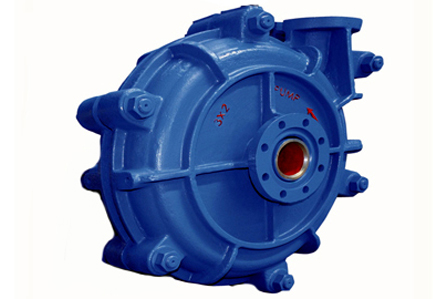
The mud pump studied in this study is a double wall centrifuge pump, including driving system, flushing system, lubrication system, water sealing system, and pressure and air control system. Its composition and structure are shown in Figure 1. The cover plate seals the suction side of the outer pump casing and is connected to the inner pump casing through bolts and nuts. Additionally, the impeller is installed in the inner pump casing, and the mud is transported through the rotation of the impeller. In addition, the impeller is connected to the pump shaft through a multi-thread thread, and the end of the pump shaft is connected to the coupling of the mud pump motor or gearbox, thereby driving the impeller to rotate. The MPWSS consists of an inner pump casing (including impeller and flow channel) and an outer pump casing (including water chamber and shaft seal). The outer pump casing connects the inner pump casing and the bearing body base and seals the inner pump casing from the shaft side. There is a pressure balance chamber between the inner and outer pump casings to ensure that the internal and external pressures are balanced and are the same as the working pressure of the mud pump.
During the operation of the mud pump, mud is transported from the low-pressure area to the high-pressure area through the stirring of the impeller. Nevertheless, the small gap between the impeller and the pump casing can cause mud to flow back towards the center of the impeller. To prevent this, sealing devices are installed on both the pump shaft side and the suction side; the shaft seal is installed at the inlet of the water chamber to prevent water and mud from entering the bearing body.
However, the transportation of mud by the pump can lead to wear on its flow-passing components. Excessive wear on the outer side of the impeller, lining plate, pump shaft seal and suction seal can result in enlarged clearance, increased backflow, and even leakage from the pump, as depicted in Figure 2. This, in turn, can lead to a significant reduction in the mud pump’s performance, necessitating frequent maintenance and parts replacement, increased operating costs, and reduced effective operating time.
Hence, the primary objective of the MPWSS is to prevent mud or slurry from entering the pump shaft seal, suction seal, and the gap between the impeller and pump shell lining of the mud pump, thereby reducing the wear of these parts and extending their service life. Furthermore, the main functions of MPWSS are as follows: (1) protecting and lubricating the shaft seal device of the mud pump; (2) protecting and lubricating the suction seal of the mud pump; (3) introducing balance water between the inner and outer pump casings to extend the service life of the inner pump casing of the mud pump.
This section presents the prediction of shaft seal water pressure in MPWSS and provides an overview of the overall framework, as demonstrated in Figure 3. This process begins with dataset input into the model, followed by data preprocessing, which involves the removal of non-relevant data points, the smoothing of abnormal points and normalization. Subsequently, a combination of key index analysis and a stacked model is used to select key characteristic parameters with high correlations. In order to reduce the adverse effects of multi-scale data on the embedding layer, the third stage is to input the data into MCNN models and generate a new time series dataset. Afterward, the generated data are aggregated into the embedding layer of the transformer model for prediction. Finally, the prediction results from these models are compared and evaluated. The main research in this chapter is data cleaning and feature selection.
To validate the prediction of shaft seal water pressure under the introduced algorithm, the research data are sourced from the construction data of the “Hua An Long” CSD on 1 November 2022. These data comprises 97 dimensions(columns) from 18:00:20 to 23:59:58 BJT. Seventy percent of the dataset is partitioned randomly for training the machine learning model, with the remaining thirty percent reserved for model performance assessment. An illustrative sample of the system monitoring data from CSD is presented in Table 1.
Before training the algorithm, it is necessary to filter out data from non-dredging operations and abnormal data, which can guarantee the efficacy of the training dataset. To achieve this, three rules are proposed for defining and distinguishing non-dredging operations and abnormal data: (1) Sensing parameters unrelated to dredging, including direction; (2) Data recorded during the start and end stages. Figure 4 illustrates the changes in the shaft seal water pressure of the underwater pump and 1# pump during the entire operation process. Specifically, subfigures 1 and subfigure 4 and 5 represent the start and end state of dredging respectively. It is worth to mentioning that the complete dredging process is divided into three stages: the initial stage, the operation stage and the finish stage. The initial stage and the finish stage belong to the non-dredging state, and their values transition from 0 to stable value and then back to 0. Thus, this part of the data can be removed; (3) Images 2 and 3 in Figure 4 are during the operation and the data theoretically belongs to the dredging operation stage, but their value changes suddenly and irregularly. Thus, this part of the value can be deleted or interpolated. To be more specific, in the algorithm of abnormal data processing, firstly, the upper and lower quartiles (Q 1 and Q 3) of each column of data were calculated. Then, the interquartile range (IQR) was calculated as Q 1–Q 3, and the threshold for outliers was defined as 1.5. Then, the lower and upper bounds for determining outliers were calculated as follows:
L o w e r B o u n d=Q 1+threshould×I Q R
(1)
U p p e r B o u n d=Q 3+threshould×I Q R
(2)
Finally, outliers were removed within the upper and lower limits. Taking one monitoring point (Shaft seal water pressure) of CSD as an example, this method effectively detects the outlier and remove it, this process can be summarized as Figure 5.
The construction data features for CSD originate from diverse sources, exhibiting varying dimensions, orders of magnitude, and significant disparities in their scales, making them unsuitable for direct computation. Hence, the application of normalization is typically an essential preprocessing step in machine learning.
This study focuses on predicting shaft end seal water pressure, which is a representative multi-input single-output prediction model. To ensure precision and facilitate comparison, normalization is necessary to standardize dimension and span variations. Normalization can be expressed as Equation (3).
x′=x−minX maxX−minX×b−a+a
(3)
where x is the original data point, min(X) and max(X) are the minimum and maximum value of all data points in the data set, respectively, a and b are the minimum and maximum values of the target range. In this research, the values should be normalized to between 0 and 1; b is 1 and a is 0. The normalized images of D2, D3, and target are shown in Figure 6. (D2 is 1# mud pump shaft seal water pressure, D3 is 1# mud pump suction seal water pressure, and target is underwater pump shaft seal water pressure).
As presented in Table 1, CSD generates an extensive array of monitoring datasets. Therefore, feature selection is a critical step before model application. Traditional data-driven techniques like maximum information coefficient (MIC) and F-tests, while effective, are susceptible to the fluctuating and complex operating conditions of CSDs, particularly when dealing with numerous sensor datasets. In response, this study proposes to combine the MPWSS key index selection method with the stacked feature selection algorithm model based on RF and XGBoost. Initially, this paper introduces the MPWSS key index selection method for initial data dimensionality reduction. This approach is based on comprehensive expert experience and prior knowledge of CSD underwater pump mechanics. It establishes a set of standards for the selection of key indices related to shaft seal water pressure. The chosen key indices prioritize real-time responsiveness, functional significance, and high data quality. Therefore, based on the construction technology of CSD, the operational principles of the MPWSS, and the most relevant key indicators during CSD construction, the following standards were established:
(1) As shown in Figure 7, the cutting system of a cutter suction dredger comprises a front-end device, a cutter, a cutter shaft, a cutter bearing box, a gearbox, a motor, an underwater pump, and a dredger pipe. This system controls cutter movement, and the mixture of mud and water produced by cutting the soil is collected through the suction inlet and dredger pipe. Therefore, based on expert experience, it can be concluded that cutter speed, cutter bearing flushing pressure, motor indicators (power, voltage, current), and traverse speeds are correlated with mud flow rate and concentration, influencing shaft seal water pressure. In summary, these parameters collectively constitute “cutter-related indices” that significantly impact shaft seal water pressure.
(2) The mud pump is the core device of the dredger operation. To prevent sediment from entering the pump shaft and causing damage during operation, the seal water pump, as depicted in Figure 1, injects water into the shaft and suction end of the mud pump. Water is injected into the pump shaft seal with specific pressure to ensure that the seal pressure exceeds the pump chamber pressure. Consequently, the seal water entering the mud pump from the pump shaft seal flows along the impeller clearance into the pump chamber, preventing mud from entering the impeller clearance and pump shaft seal. Additionally, a CSD typically includes at least one underwater pump, with larger CSDs featuring 1–2 additional pumps for pressurization. Therefore, the most relevant indices related to the mud pump are those generated by the pump itself. Finally, this study introduces “pump-related indices”, including suction vacuum, rotation speed, pump power, pump torque, shaft drive power, suction end seal water pressure, 1# pump and 2# pump shaft seal water pressure, and pump discharge pressure.
(3) As shown in Figure 8, during the dredging process of the CSD, the cutter cuts through the underwater silt rock layer, and the mud is extracted through the vacuum created by the underwater pump. Subsequently, it is transported to the filling area via the mud suction and discharge pipeline. Due to the considerable length of the pipeline, two additional centrifugal pumps (1# pump and 2# pump) are necessary for pressurization to ensure the transportation of all the mud to the mud outlet. Consequently, certain indicators directly pertain to the mud flow rate and pressure of the underwater pump, while others exhibit indirect relationships, subsequently influencing the water pressure at the shaft end of the underwater pump. As a result, this paper proposes the introduction of “mud transportation-related indices”, including suction vacuum level, mud flow rate, mud concentration, outlet flow rate, and productivity.
Through conducting initial MPWSS key index selection filtering, relevant characteristic parameters can be preliminarily identified. Afterward, two intelligent algorithms Random Forest and XGBoost were combined, and the weights were set to 0.5 respectively. This stacked model provides a more comprehensive assessment of feature importance and resolves the overfitting problem that may exist in a single model. Based on this stacked model, the 25 features with the highest comprehensive importance ranking are extracted, as shown in Figure 9. As can be seen from the figure, the parameter “Current shift output” has the highest correlation coefficient. This parameter indicates the current working status of the motor. Since there is a mechanical or hydraulic transmission relationship between the underwater pump and the motor, the greater the load on the motor, the greater the load on the pump and the output pressure may be higher, resulting in greater sealing water pressure required. The second most relevant parameter is “tide level”. The tidal water level changes periodically, so the output pressure of the underwater pump may also change periodically. When the tidal water level is high, the underwater pump requires a higher speed. To pump mud from deeper waters, higher sealing water pressures may need to be generated.
This study selected the 25 parameters with the highest correlation and conducted comparative analysis with other parameters with lower correlation coefficients. The location distribution of related sensors on the ship and their mutual influence are shown in Figure 10. It can be seen from this figure that the underwater pump has a physical connection with some sensors, which means a certain mathematical formula, and also has a data connection with some sensors, which means there is a certain correlation calculated through Random Forest and XGBoost algorithms.
In this section, 25 features that are highly relevant to the MPWSS of CSD were selected according to the MPWSS key index selection method and stacked model. Furthermore, the MCNN-transformer model is introduced and six other representative models are selected through comparative analysis to predict the data, and conduct a comparative analysis of the root mean mquare error (RMSE), mean absolute error (MAE), MAPE (Mean Absolute Percentage Error) and coefficient of determination (R 2) of each model.
CNN is a classic deep-learning algorithm. However, in this study, the input covers 25 parameters that are correlated with the output. MCNN focuses on the extraction of multi-scale features, and its structure usually contains multiple parallel convolution and pooling layers. Each layer focuses on feature extraction at different scales, which helps capture feature information of different targets. The overall structure of MCNN is shown in Figure 11. The multi-scale convolution module in Figure 11 uses three convolution layers with different convolution kernel sizes to extract multi-scale features of the input data. The outputs of these feature extraction layers are further fed into the fourth fusion convolutional layer for feature fusion operations. Finally, the features processed by a deep convolutional model are transferred into the fully connected layer to produce the final output result.
In the convolutional layer, the mathematical form of the convolution operation can be expressed as Equation (4):
X O=∑X I×W l+b l
(4)
where X O is the convolution calculation result, X I is the input of the previous layer, and W l and b l are the weight and bias terms of the l t h convolutional layer respectively.
The kernel_size, padding and stride of each Conv_block are illustrated Figure 11. For example, in Conv_block1, the kernel_size is 2, the padding is 3, and the stride is 2. This model uses BatchNorm2d for normalization, rectified linear unit (ReLU) as activation function in the convolution block and fully connected layer, and SoftMax activation function in the output layer.
The transformer model was first proposed by Vaswani in 2017. The core idea of the Transformer model is to completely abandon the structure of the traditional recurrent neural network (RNN) and convolutional neural network (CNN), and instead apply the self-attention mechanism (self-attention mechanism). The Transformer model consists of two parts: the encoder and the decoder. Each layer contains a multi-head self-attention mechanism and a feedforward neural network, as depicted in Figure 12. The multi-head attention mechanism allows the model to pay attention to different semantic representation subspaces at the same time. Moreover, the transformer model also introduces positional encoding to process the position information of the sequence, as well as residual connection and layer normalization technology to stabilize the training process.
Input the feature sequence generated by MCNN into the embedding layer of the transformer model. In the positional encoding part, model utilizes the sine and cosine functions to encode the positional information, as shown in Equations (5) and (6):
P E p o s,2 i=sinp o s 10,000 2 i d
(5)
P E p o s,2 i+1=cosp o s 10,000 2 i d
(6)
where p o s represents the position and i is the dimension, i∈(0,d 2). A vector is created using the cosine function for odd positions and a sine function for even positions, and then these vectors are added to the corresponding embedding vectors.
As shown in Figure 12, it is the framework of the multi-head attention mechanism. The multi-head attention mechanism is based on the self-attention mechanism. In the self-attention mechanism, the input is fed into three different fully connected Linear layers to create query, key and value. Query and key are multiplied by dot product matrix to generate a score matrix of scores. Then the scores matrix is processed, and the process can be expressed as Equation (7):
s c o r e s d k=s c a l e s c o r e s
(7)
Then SoftMax calculation is performed on the scaled scores to obtain the attention weight. Finally, the attention weight is multiplied by the value vector to obtain the final output vector. The output of self-attention can be expressed as Equation (8):
A t t e n t i o n Q,K,V=S o f t M a x Q K T d k V
(8)
where Q∈R T×d, K∈R T×d and V∈R T×d. The SoftMax function can be expressed as Equation (9):
S o f t M a x z i=e z i∑j=1 k e z j
(9)
where z i is the i t h element in the input vector, and K is the dimension of the vector. The SoftMax function performs an exponential operation on each element in the input vector and then divides each exponential value by the sum of all exponential values, resulting in a probability distribution with each element in the range [0, 1].
To extend the calculation to multi-head attention, the query, key, and value vectors need to be divided into n vectors before applying the self-attention mechanism. Subsequently, these divided vectors undergo the aforementioned self-attention mechanism. Each self-attention process is referred to as a “head”, and each head produces an output vector. The n heads are calculated in parallel and then combined to generate the output, constituting the multi-head attention mechanism. The formula of multi-head attention is expressed as Equations (10) and (11).
M u l t i H e a d Q,K,V=C o n t a c t h e a d 1,h e a d 2,h e a d 3,…,h e a d n W O
(10)
h e a d i=A t t e n t i o n Q W i Q,K W i K,V W i Q V
(11)
where i=1,2,3,4,…,h, W O, W i Q, W i K and W i V are the weights of corresponding networks, W O∈R d m o d e l×d k, W i Q∈R d m o d e l×d k, W i K∈R d m o d e l×d k and W i V∈R d m o d e l×d v. Contact function is the splicing of results generated by parallel calculation of all heads.
As shown in Figure 13, the feedforward neural network consists of two linear transformation layers and a nonlinear activation function (ReLU). FFN accepts the signal from the multi-head attention layer, and maps the input vector to a higher dimensional space through two linear transformation layers, followed by a nonlinear transformation through the activation function to finally obtain a new output, which ensures that the model can learn more complex features. The calculation process of FFN can be expressed as Equation (12):
Y=R e L U x W 1+b 1 W 2+b 2
(12)
where the input vector is x; the output vector is Y; W 1 and W 2 are the weight matrix of the first and second linear transformations, and b 1 and b 2 are the bias vector.
The normalization layer helps alleviate the problems of vanishing and exploding gradients, and usually follows the output of each sub-layer (such as multi-head self-attention mechanisms and feedforward neural networks).
The original transformer model first converts a single moment sample in the input sequence into a high-dimensional feature vector through the embedding layer, and then applies positional encoding to process the information of each position in the sequence. Subsequently, the multi-head attention mechanism is used to map the input features into three feature vectors: query (Q), key (K) and value (V). Through computing the correlation between the query (Q) and the key (K), the values (V) are subsequently weighted and summed to generate the features of the next time step.
However, the prediction of underwater pump shaft seal water pressure is a regression prediction problem. Since the embedding layer of the transformer model is not suitable for feature extraction of multi-time series data, the original model needs to be optimized. In this study, an MCNN-transformer model is proposed, Figure 13 illustrates the details of model. The original data sequence is input into MCNN and multi-scale features are extracted. Subsequently, these feature sequences are input into the embedding layer of the Transformer model, and the self-attention mechanism of the Transformer model is used to model the global relationship of the sequences. The advantage of this dual model combination is that MCNN can effectively extract multi-time scale local features from the original data, while Transformer can understand and model sequence data on a global scale, thus improving the performance of the model in processing complex sequence data.
To quantitatively evaluate and compare the predictive accuracy of each model, this study employs three evaluation indices: the root mean square error (RMSE), mean absolute error (MAE), MAPE (Mean Absolute Percentage Error) and the Coefficient of determination (R 2).
(1) Root mean square error (RMSE)
R M S E=1 N∑t=1 N Y O−Y P 2
(13)
(2) Mean absolute error (MAE)
M A E=∑t=1 N Y O−Y P N
(14)
(3) MAPE (Mean Absolute Percentage Error)
M A P E=100%n×∑i=1 N y i^−y i y i
(15)
(4) Coefficient of determination (R 2)
R 2=1−∑i=1 N y i^−y i 2∑i=1 N y i¯−y i 2
(16)
The root mean square error (RMSE) measures the square root of the average squared differences between predicted and actual values, providing a sense of scale for prediction errors, which can be expressed as Equation (13). Mean absolute error (MAE) represents the average magnitude of prediction discrepancies, emphasizing the absolute error magnitude, which can be expressed as Equation (14). If MAPE = 0%, the model is a perfect model, and MAPE greater than 100% indicates an inferior model. The smaller the value of MAPE, the better the accuracy of the prediction model, which can be expressed as Equation (15), MAPE∈[0,+∞]. The coefficient of determination (R 2) evaluates the proportion of variance in the dependent variable that the model explains. The closer the value of R 2 is to 1, the better the fit of the regression line to the observed values, which can be expressed as Equation (16), R 2∈[0,1].
In order to verify the performance of the MCNN transformer model in predicting shaft seal water pressure, it was compared with the MCNN, transformer, RF, BP and XGBoost prediction models. For the MCNN transformer model, the MCNN method is employed to process various types of input data. Through multi-layer convolution operations, it captures features from the time series data. The extracted time series features are then enhanced and transformed to improve feature representation and the model’s generalization ability. Additionally, the MCNN model reconstructs the time series data and converts them into the input format processed by the embedding layer of the Transformer model.
In addition, this study compares the hybrid model MCNN-Transformer with single models including MCNN, transformer, Random Forest, CNN, BP, and XGBoost. To assess the prediction performance of these models, four commonly used evaluation indexes, R 2, MAE, MSE, and MAPE, are employed. Moreover, time is considered one of the evaluation criteria for assessing the timeliness of the models. The prediction results are presented in Table 2. Through observing and analyzing the evaluation indicators of the seven models, it is evident that the MCNN transformer model exhibits the highest coefficient of determination (R 2), while the errors (MAE, MSE, MAPE) between the predicted and actual values are the smallest. In order to visually represent the relationship between the evaluation indicators of each model more intuitively, we have plotted the radar chart of these seven models, as shown in Figure 14.
By analyzing Table 2 and integrating findings from actual dredging engineering research, we can draw conclusions on how to effectively and appropriately integrate artificial intelligence technology with dredging engineering.
(1) It is obvious that the MCNN transformer model achieved the best performance, with the highest coefficient of determination of 0.9624, lowest MAE of 0.0108, MAPE of 0.0051 and MSE of 0.00018. On the contrary, the traditional single neural network model Random Forest (RF) obtains the worst performance, with the lowest coefficient of determination of 0.8078, highest MAE of 0.0247, MAPE of 0.0118 and MSE of 0.00094.
(2) Compared to a single transformer model, the hybrid model employs the MCNN model for data convolution before inputting datasets into the transformer model which has indeed enhanced the predictive performance. However, the time required for the MCNN transformer model to predict the shaft end sealing water pressure is 23.93 s, approximately three times longer than that of the Transformer model.
(3) For dredging projects, if the pressure sensor of the MPWSS fails during the construction process, to ensure that the mud pump can operate normally and continuously, it is necessary to quickly restore the sensing data of the shaft seal water pressure. The shortest time-consuming model the XGBoost model could be used for prediction. In comparison, this model takes the shortest time to predict, only 0.02 s, but it has a coefficient of determination of 0.8455. However, if the wear of the mud pump is serious during construction, a model with higher accuracy and shorter time consumption is essential. It is recommended to use the CNN model, which, with a prediction time of 4.95 s, remains within an acceptable timeframe while offering significantly higher prediction accuracy, up to 0.9431.
(4) In some common dredging construction areas, if a pressure sensor failure causes the mud pump water sealing system to fail to work properly, experienced operators can still increase the sealing water pressure as much as possible to minimize the wear of the mud pump. In such cases, the calculation time requirement is not strict, but it is crucial to accurately sense the seal water pressure required by the mud pump and understand its current working conditions. Therefore, it is recommended to utilize the MCNN transformer model.
To further illustrate the experimental comparison results of the seven proposed models, Figure 15 shows the prediction curves of all models on the test set, Figure 16 shows the prediction curve of the MCNN transformer model, and Figure 17 shows the prediction curve of the remaining six models. By observing the partially enlarged picture, it can be clearly seen that the MCNN transformer model proposed in this study can fit the test data better. The parameters in the figure generally fluctuate within a certain range, indicating that the construction status of the mud pump is good and the soil properties are stable. A certain section is selected in the
Bookmark
Daniel Féau processes personal data in order to optimise communication with our sales leads, our future clients and our established clients.


This site is protected by reCAPTCHA and the Google Privacy Policy and Terms of Service apply.